
Each quarter the backup service BackBlaze publishes data on the failure rate of its hundreds of thousands of hard drives, most recently on February 11th. Since the failure rate of different models can vary widely, these posts sometimes make a splash in the tech community. They’re also notable as the only large public dataset on drive failures:
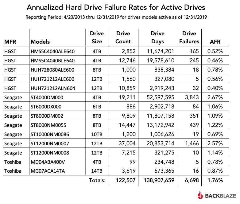
One of the things that strikes me about the presentation above is that BackBlaze uses simple averages to compute the “Annualized Failure Rate” (AFR), despite the fact that the actual count data vary by orders of magnitude, down to a single digit. This might lead us to question the accuracy for smaller samples; in fact, the authors are sensitive to this possibility and suppress data from drives with less than 5,000 days of operation in Q4 2019 (although they are detailed in the text of the article and available in their public datasets).
This looks like a perfect use case for a Bayesian approach: we want to combine a prior expectation of the failure rate (which might be close to the historical average across all drives) with observed failure events to produce a more accurate estimate for each model.
Re-estimating Failure Rates using Empirical Bayes
First, we can extract the data that is missing from the table but mentioned in the text:
(omitted <- tibble::tribble(
  ~mfg, ~name, ~size, ~days, ~failures,
  "Seagate", "ST16000NM001G", "16TB", 1440, 0,
  "Toshiba", "HDWF180", "8TB", 13994, 1,
  "HGST", "HUH721010ALE600", "10TB", 8042, 0,
  "Toshiba", "MG08ACA16TA", "16TB", 100, 0,
))
#> # A tibble: 4 x 5
#>   mfg     name            size   days failures
#>   <chr>   <chr>           <chr> <dbl>    <dbl>
#> 1 Seagate ST16000NM001G   16TB   1440        0
#> 2 Toshiba HDWF180         8TB   13994        1
#> 3 HGST    HUH721010ALE600 10TB   8042        0
#> 4 Toshiba MG08ACA16TA     16TB    100        0
You’ll notice that there are zero failures for most of these drives, even though it seems implausible that they will never fail. This approach will allow us to fill in reasonable estimates.
The remaining data come from the CSV download available in the original post, cleaned up a little:
fname <- "path/to/lifetime_chart_as_of_Q4_2019.csv"
library(dplyr, warn.conflicts = FALSE)

hdds <- read.csv(
  fname, skip = 4, row.names = NULL, stringsAsFactors = FALSE,
  nrows = 14
) %>%
  tibble::as_tibble() %>%
  select(
    mfg = MFR, name = Models, size = Drive.Size, days = Drive.Days,
    failures = Drive.Failures
  ) %>%
  mutate(
    name = trimws(gsub(",", "", name, fixed = TRUE)),
    days = as.integer(gsub(",", "", days, fixed = TRUE)),
    failures = as.integer(gsub(",", "", failures, fixed = TRUE))
  ) %>%
  bind_rows(omitted) %>%
  mutate(
    # Compute BackBlaze's "Annualized Failure Rate".
    afr = failures / (days / 365)
  ) %>%
  arrange(desc(afr))

hdds
#> # A tibble: 18 x 6
#>    mfg     name            size      days failures     afr
#>    <chr>   <chr>           <chr>    <dbl>    <dbl>   <dbl>
#>  1 Seagate ST4000DM000     4TB   52597595     3843 0.0267
#>  2 Toshiba HDWF180         8TB      13994        1 0.0261
#>  3 Seagate ST12000NM0007   12TB  20853714     1466 0.0257
#>  4 Seagate ST8000NM0055    8TB   13172942      439 0.0122
#>  5 Seagate ST12000NM0008   12TB    321275       10 0.0114
#>  6 Seagate ST8000DM002     8TB   11807158      351 0.0109
#>  7 Seagate ST6000DX000     6TB    2902718       84 0.0106
#>  8 Toshiba MG07ACA14TA     14TB    673365       16 0.00867
#>  9 HGST    HUH728080ALE600 8TB     838384       18 0.00784
#> 10 Toshiba MD04ABA400V     4TB     234748        5 0.00777
#> 11 Seagate ST10000NM0086   10TB   1006626       19 0.00689
#> 12 HGST    HUH721212ALE600 12TB    327080        5 0.00558
#> 13 HGST    HMS5C4040ALE640 4TB   11674201      165 0.00516
#> 14 HGST    HMS5C4040BLE640 4TB   19578610      245 0.00457
#> 15 HGST    HUH721212ALN604 12TB   2919243       32 0.00400
#> 16 Seagate ST16000NM001G   16TB      1440        0 0
#> 17 HGST    HUH721010ALE600 10TB      8042        0 0
#> 18 Toshiba MG08ACA16TA     16TB       100        0 0
David Robinson has a well-known blog post on an analogous problem in baseball where he takes an empirical Bayes approach and estimates a reasonable prior distribution from the original data – which works here as well. To get a more stable estimate of the distribution, we can omit AFRs computed for drives with less than 1 million days of service:
afr_sample <- hdds$afr[hdds$days > 1e6]
(afr_beta <- MASS::fitdistr(
  afr_sample, dbeta, start = list(shape1 = 1.5, shape2 = 100),
  lower = 0.01
))
#>      shape1       shape2
#>     2.379848   198.621649
#>  (  1.052762) ( 97.652075)

# Empirical beta prior parameters.
alpha0 <- afr_beta$estimate[1]
beta0 <- afr_beta$estimate[2]
This models the failure rate of each model as fixed but drawn from a shared beta distribution (which is a natural distribution for probabilities), and individual days as a Bernoulli trial that can either succeed or fail based on this underlying rate. This is a contestable model – for instance, you might think that workload or other environmental factors are the true cause of failures – but I believe it’s a reasonable approximation.
With the parameters in hand we can then use Bayes rule to update the rates1, combining the empirical prior with the observed data:
mutate(
  hdds, eb_afr = (failures + alpha0) / ((days / 365) + alpha0 + beta0)
)
#> # A tibble: 18 x 7
#>    mfg     name            size      days failures     afr  eb_afr
#>    <chr>   <chr>           <chr>    <dbl>    <dbl>   <dbl>   <dbl>
#>  1 Seagate ST4000DM000     4TB   52597595     3843 0.0267  0.0266
#>  2 Toshiba HDWF180         8TB      13994        1 0.0261  0.0141
#>  3 Seagate ST12000NM0007   12TB  20853714     1466 0.0257  0.0256
#>  4 Seagate ST8000NM0055    8TB   13172942      439 0.0122  0.0122
#>  5 Seagate ST12000NM0008   12TB    321275       10 0.0114  0.0115
#>  6 Seagate ST8000DM002     8TB   11807158      351 0.0109  0.0109
#>  7 Seagate ST6000DX000     6TB    2902718       84 0.0106  0.0106
#>  8 Toshiba MG07ACA14TA     14TB    673365       16 0.00867 0.00898
#>  9 HGST    HUH728080ALE600 8TB     838384       18 0.00784 0.00816
#> 10 Toshiba MD04ABA400V     4TB     234748        5 0.00777 0.00874
#> 11 Seagate ST10000NM0086   10TB   1006626       19 0.00689 0.00723
#> 12 HGST    HUH721212ALE600 12TB    327080        5 0.00558 0.00673
#> 13 HGST    HMS5C4040ALE640 4TB   11674201      165 0.00516 0.00520
#> 14 HGST    HMS5C4040BLE640 4TB   19578610      245 0.00457 0.00459
#> 15 HGST    HUH721212ALN604 12TB   2919243       32 0.00400 0.00419
#> 16 Seagate ST16000NM001G   16TB      1440        0 0       0.0116
#> 17 HGST    HUH721010ALE600 10TB      8042        0 0       0.0107
#> 18 Toshiba MG08ACA16TA     16TB       100        0 0       0.0118
If you look carefully, you’ll see that drives with smaller samples are more strongly influenced by the prior: all of the drives that were originally omitted have failure rates close to the mean of the prior, and the model suggests that some of the large HGST drives have had a run of good luck as well.
Of course, a plot (see the top of the page) is more compelling than a table.
There is some evidence in the table above that different manufacturers may have slightly different base failure rates, and BackBlaze has in the past speculated that different drive sizes may have different failure characteristics as well. In this case, you could try to recover manufacturer- or drive size-specific parameters by using a hierarchical model. This approach might bring the estimate for the HGST 10TB drive down, for example, since the other HGST models all have low failure rates.
Finally, it’s worth mentioning that failure rates in and of themselves may not be the right metric against which to make a purchasing decision – the drives vary in size and price, so a more useful measure might be an estimate of the annual per-TB replacement cost for each model.
-
This simple update formula for the beta-binomial is due to the highly convenient fact that the posterior distribution is also beta-binomial, which is partly why this distribution is so popular. ↩︎